Keras environment.
We will use a Kaggle Dataset in which there are 32 topics and more than 400K total reviews.
If you would like to learn more about Deep Learning with practical coding examples,
Please subscribe to the Murat Karakaya Akademi YouTube Channel or
Follow my blog on muratkarakaya.net
Do not forget to turn on notifications so that you will be notified when new parts are uploaded.
You can access all the codes, videos, and posts of this tutorial series from the links below.
Accessible on:
YouTube in English
YouTube in Turkish
muratkarakaya.net
Github pages
Github Repo
Google Colab

PARTS
In this tutorial series, there are several parts to cover Text Classification with various Deep Learning Models topics. You can access all the parts from this index page.

In this part, we will use the Keras Bidirectional LSTM layer in a Feed Forward Network (FFN).

If you are not familiar with the Keras LSTM layer or the Recurrent Networks concept, you can check in the following Murat Karakaya Akademi YouTube playlists:

English:

All About LSTM

Turkish

LSTM hakkında herşey!

If you are not familiar with the classification with Deep Learning topic, you can find the 5-part tutorials in the below Murat Karakaya Akademi YouTube playlists:

Photo by Markus Spiske on Unsplash

Part G: Text Classification with A Recurrent Layer

Let’s build a model with a Bidirectional LSTM layer

Important LSTM Parameters

I would like to kindly remind you of the important parameters in the Keras LSTM layer briefly. For more information, you can visit the Keras official documentation here.

tf.keras.layers.LSTM(
    units,
    return_sequences=False,
    return_state=False,
    
)

units: Positive integer, the dimensionality of the output space. In other words, it sets the number of output units or nodes in the layer. This is a required parameter.
return_sequences: Boolean. Whether to return the last output in the output sequence or the full sequence. Default: False. If set to True, the layer will return the full sequence of outputs, which is useful if you are stacking multiple LSTM layers. If set to False (the default), the layer will only return the last output, which is useful for tasks such as predicting a single output value.
return_state: Boolean. Whether to return the last state in addition to the output. Default: False. If set to True, the layer will return a list of the final hidden state and final cell state, which can be useful for initializing the state of a subsequent LSTM layer. If set to False (the default), the layer will only return the output.

In our model, I will use an LSTM layer with the following parameters and their values:

units= 256
return_sequences= True

LSTM(256, return_sequences=True)

Why do we set return_sequences parameter to true?

In the given model, the return_sequences parameter of the Bidirectional LSTM layer is set to True. This means that the layer will return the full sequence of outputs for each timestep instead of just the last output.

There are a few reasons why return_sequences=True might be used in a model. In this case, we set it true, because we want to use the LSTM layer for feature extraction. In some cases, like text classification, LSTM layers can be used to extract features from sequential data (here: tokens). By setting return_sequences=True, you can extract features from every timestep of the input sequence (here are the tokens from a review) and use them as inputs to subsequent layers.

Lastly, the shape of this layer’s output will be (time-steps,256). Remember that, in our previous tutorials, we set the sequence size fix to 40 tokens. Therefore, the number of time steps is 40.

Why do we use Bidirectional LSTM?

Furthermore, we chose to use Bidirectional LSTM by adding the Biderectional layer.

x = layers.Bidirectional(layers.LSTM(256, return_sequences=True))(x)

The bidirectional LSTM layer in the model is used to capture both forward and backward context in the input sequence. This is particularly useful in natural language processing tasks such as text classification because the meaning of a word can depend on the words that come before and after it in the sentence.

A standard LSTM layer can only capture the context in one direction, either forward or backward, but not both at the same time. In contrast, a bidirectional LSTM layer processes the input sequence in both directions, allowing it to capture context from both directions and provide a more complete understanding of the input sequence.

Using a bidirectional LSTM layer can lead to better performance on text classification tasks because it can capture more complex dependencies in the input sequence, which is important for accurate classification. It also allows the model to learn features that are not just based on the previous context of the input sequence, but also on the future context.

Therefore, a bidirectional LSTM layer is a common choice for text classification tasks where the input sequence has complex dependencies that require the model to capture context from both directions.

If you would like to conduct an experiment just remove the bidirectional layer, retrain the model, and observe the performance. You would see that the model without a bidirectional layer will perform very poorly.

The image is taken here

Because of Bidirectional LSTM, the shape of the output from these layers becomes (time-steps,2*256) = (40, 512). You will observe this output shape in the following model summarization below.

Here is a sample Feed Forward NN model with a Bidirectional LSTM layer. The details of the model are given below per layer.

embed_dim = 16  # Embedding size for each token
feed_forward_dim = 64  # Hidden layer size in feed forward network 

def create_model_LSTM():
    inputs_tokens = layers.Input(shape=(max_len,), dtype=tf.int32)
    embedding_layer = layers.Embedding(input_dim=vocab_size, 
                                       output_dim=embed_dim, 
                                       input_length=max_len)
    x = embedding_layer(inputs_tokens)
    #x = layers.LSTM(, activation='relu',return_sequences=True)(x)
    x = layers.Bidirectional(layers.LSTM(256, return_sequences=True))(x)
    x = layers.Dropout(0.2)(x)  
    x = layers.Dense(feed_forward_dim, activation='relu')(x)
    x = layers.GlobalMaxPool1D()(x)
    outputs = layers.Dense(number_of_categories)(x)
    model = keras.Model(inputs=inputs_tokens, 
                        outputs=outputs, name='model_LSTM')
    loss_fn = tf.keras.losses.SparseCategoricalCrossentropy(from_logits=True)
    metric_fn  = tf.keras.metrics.SparseCategoricalAccuracy()
    model.compile(optimizer="adam", loss=loss_fn, metrics=metric_fn)  
    
    return model
model_LSTM=create_model_LSTM()time: 2.2 s (started: 2023-03-24 13:26:43 +00:00)

In the above code:

inputs_tokens = layers.Input(shape=(max_len,), dtype=tf.int32) creates an input layer for the model that expects integer sequences of length max_len. Note that in our tutorial series max_len is 40 tokens.
embedding_layer = layers.Embedding(input_dim=vocab_size, output_dim=embed_dim, input_length=max_len) creates an embedding layer that maps each token in the input sequence to a dense vector of size embed_dim. This layer will learn the vector representations of the tokens during training. Here, we set embed_dim as 16, max_len is 40 tokens, and vocab_size is 100K tokens.
x = embedding_layer(inputs_tokens) applies the embedding layer to the input sequence, resulting in a tensor of shape (batch_size, max_len, embed_dim).
x = layers.Bidirectional(layers.LSTM(256, return_sequences=True))(x) adds a bidirectional LSTM layer to the model such that output dimension is 2*256. The return_sequences=True argument means that the layer will return the full sequence of outputs at each time steps (we have 40 tokens) rather than just the final output.
x = layers.Dropout(0.2)(x) adds a dropout layer that randomly sets 20% of the input units to 0 during training. This helps prevent overfitting by adding noise to the network.
x = layers.Dense(feed_forward_dim, activation='relu')(x) adds a feedforward layer with feed_forward_dim hidden units and ReLU activation function.
x = layers.GlobalMaxPool1D()(x) applies a global max pooling operation to the output of the feedforward layer. This reduces the tensor to a one-dimensional tensor of shape (batch_size, feed_forward_dim).
outputs = layers.Dense(number_of_categories)(x) adds a dense layer with number_of_categories units, which will be the output layer of the model. The output layer produces a probability distribution over the possible classes.
model = keras.Model(inputs=inputs_tokens, outputs=outputs, name='model_LSTM') creates a Keras model with the input and output layers defined above.
loss_fn = tf.keras.losses.SparseCategoricalCrossentropy(from_logits=True) creates a loss function that calculates the cross-entropy loss between the predicted and true labels. The from_logits=True argument means that the output of the model is not normalized into a probability distribution, so the loss function will apply the softmax function internally.
metric_fn = tf.keras.metrics.SparseCategoricalAccuracy() creates a metric function that calculates the accuracy of the model predictions.
model.compile(optimizer="adam", loss=loss_fn, metrics=metric_fn) compiles the model with the Adam optimizer, the cross-entropy loss function, and the accuracy metric function.

Let’s see a summary and plot of the model. Please notice the input and output shapes at each layer. If you do not understand these numbers please write a comment. I will answer them soon.

model_LSTM.summary()Model: "model_LSTM"
_________________________________________________________________
 Layer (type)                Output Shape              Param #   
=================================================================
 input_3 (InputLayer)        [(None, 40)]              0         
                                                                 
 embedding_1 (Embedding)     (None, 40, 16)            1600000   
                                                                 
 bidirectional_1 (Bidirectio  (None, 40, 512)          559104    
 nal)                                                            
                                                                 
 dropout (Dropout)           (None, 40, 512)           0         
                                                                 
 dense (Dense)               (None, 40, 64)            32832     
                                                                 
 global_max_pooling1d (Globa  (None, 64)               0         
 lMaxPooling1D)                                                  
                                                                 
 dense_1 (Dense)             (None, 32)                2080      
                                                                 
=================================================================
Total params: 2,194,016
Trainable params: 2,194,016
Non-trainable params: 0
_________________________________________________________________
time: 32.2 ms (started: 2023-03-24 13:26:49 +00:00)

Here is a quick explanation of the input/output shapes:

An input layer takes in a tensor of shape (None, 40) where None indicates a variable batch size and 40 represents the length of each input sequence (in our case 40 tokens in a review)
An embedding layer converts each integer in the input sequence into a vector of size 16. The output shape of this layer is (None, 40, 16).
A bidirectional LSTM layer processes the input sequence in both directions and returns a sequence of hidden states of size (2*256) 512. The output shape of this layer is (None, 40, 512).
A dropout layer randomly sets a fraction of the input units to zero during training to prevent overfitting.
A dense layer applies a fully connected layer with 64 units to each element in the sequence. The output shape of this layer is (None, 40, 64).
A global max pooling 1D layer takes the maximum value across the sequence dimension of the previous layer and returns a tensor of shape (None, 64). You can think of that layer as a summary (representation) of the review because we shrink the dimension from (None,40,64) to (None, 64).
A dense layer applies a fully connected layer with 32 units to the output of the previous layer. The output shape of this layer is (None, 32). Actually, this is the number of review classes. So, generally, this layer is called a classification layer.

Therefore, the input shape of the model is (None, 40) where None indicates a variable batch size and 40 represents the length of each input sequence (review). The output shape of the model is (None, 32) where None indicates a variable batch size and 32 represents the number of output units of the last dense layer (review classes).

tf.keras.utils.plot_model(model_LSTM,show_shapes=True)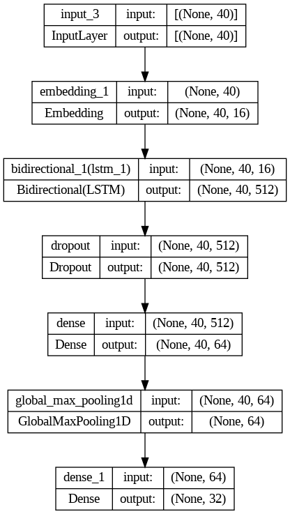

time: 1.37 s (started: 2023-03-24 13:26:56 +00:00)history=model_LSTM.fit(train_ds, validation_data=val_ds ,verbose=1, epochs=25)Epoch 1/25
237/237 [==============================] - 35s 98ms/step - loss: 3.0754 - sparse_categorical_accuracy: 0.0941 - val_loss: 2.4553 - val_sparse_categorical_accuracy: 0.2320
Epoch 2/25
237/237 [==============================] - 2s 10ms/step - loss: 1.8205 - sparse_categorical_accuracy: 0.4266 - val_loss: 1.5210 - val_sparse_categorical_accuracy: 0.5499
....Epoch 22/25
237/237 [==============================] - 3s 11ms/step - loss: 0.0023 - sparse_categorical_accuracy: 0.9995 - val_loss: 1.3712 - val_sparse_categorical_accuracy: 0.8017
Epoch 23/25
237/237 [==============================] - 3s 12ms/step - loss: 0.0018 - sparse_categorical_accuracy: 0.9996 - val_loss: 1.3314 - val_sparse_categorical_accuracy: 0.8053
Epoch 24/25
237/237 [==============================] - 3s 12ms/step - loss: 0.0031 - sparse_categorical_accuracy: 0.9994 - val_loss: 1.3111 - val_sparse_categorical_accuracy: 0.7981
Epoch 25/25
237/237 [==============================] - 2s 10ms/step - loss: 0.0050 - sparse_categorical_accuracy: 0.9989 - val_loss: 1.3708 - val_sparse_categorical_accuracy: 0.7927
time: 1min 40s (started: 2023-03-24 13:27:20 +00:00)

Looking at the output of the last three epochs, we can make the following observations:

Training loss: The training loss continues to decrease, which is a good sign that the model is learning and improving.

Training accuracy: The training accuracy is very high, which indicates that the model is fitting the training data very well.

Validation loss: The validation loss continues to fluctuate around 1.3–1.4, which is relatively high compared to the training loss. This could be an indication of overfitting, as the model may be fitting to the noise in the training data.

Validation accuracy: The validation accuracy seems to be fluctuating around 0.8, which is relatively low compared to the training accuracy. This is another indication that the model may be overfitting and not generalizing well to new, unseen data.

Based on these observations, it seems like the model may be overfitting the training data. One way to address this could be to use regularization techniques such as dropout or L2 regularization. Additionally, it may be helpful to increase the size of the validation set or use techniques such as cross-validation to better evaluate the model’s performance on new, unseen data.

I will discuss these issues in PART K: HYPERPARAMETER OPTIMIZATION (TUNING), UNDERFITTING, AND OVERFITTING.

plt.plot(history.history['sparse_categorical_accuracy'])
plt.plot(history.history['val_sparse_categorical_accuracy'])
plt.title('model_Conv1D accuracy')
plt.ylabel('accuracy')
plt.xlabel('epoch')
plt.legend(['train', 'val'], loc='upper left')
plt.show()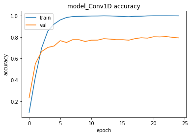

time: 284 ms (started: 2023-03-24 13:29:09 +00:00)plt.plot(history.history['loss'])
plt.plot(history.history['val_loss'])
plt.title('model_Conv1D loss')
plt.ylabel('loss')
plt.xlabel('epoch')
plt.legend(['train', 'val'], loc='upper left')
plt.show()

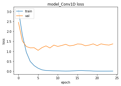
time: 202 ms (started: 2023-03-24 13:29:18 +00:00)

You can observe the underfitting and overfitting behaivors of the model and decide how to handle these situaitons by tuning the hiper-parameters.

In this tutorial, I will not go into the details of hiper-parameter tuning, underfitting and overfitting concepts. However, in PART K: HYPERPARAMETER OPTIMIZATION (TUNING), UNDERFITTING AND OVERFITTING, we will see these concepts in detail.

Save the trained model

tf.keras.models.save_model(model_LSTM, 'MultiClassTextClassification_BiLSTM')WARNING:absl:Found untraced functions such as lstm_cell_4_layer_call_fn, lstm_cell_4_layer_call_and_return_conditional_losses, lstm_cell_5_layer_call_fn, lstm_cell_5_layer_call_and_return_conditional_losses while saving (showing 4 of 4). These functions will not be directly callable after loading.


time: 15 s (started: 2023-03-24 13:29:33 +00:00)

Test

loss, accuracy = model_LSTM.evaluate(test_ds)
print("Test accuracy: ", accuracy)1319/1319 [==============================] - 17s 12ms/step - loss: 1.3494 - sparse_categorical_accuracy: 0.7985
Test accuracy:  0.7985453009605408
time: 17.2 s (started: 2023-03-24 13:29:51 +00:00)

Predictions

We can use the trained model predict() method to predict the class of the given reviews as follows:

preds = model_LSTM.predict(test_ds)
preds = preds.argmax(axis=1)1319/1319 [==============================] - 7s 5ms/step
time: 8.37 s (started: 2023-03-24 13:30:08 +00:00)

We can also get the actual (true) class of the given reviews as follows:

actuals = test_ds.unbatch().map(lambda x,y: y)  
actuals=list(actuals.as_numpy_iterator())WARNING:tensorflow:From /usr/local/lib/python3.9/dist-packages/tensorflow/python/autograph/pyct/static_analysis/liveness.py:83: Analyzer.lamba_check (from tensorflow.python.autograph.pyct.static_analysis.liveness) is deprecated and will be removed after 2023-09-23.
Instructions for updating:
Lambda fuctions will be no more assumed to be used in the statement where they are used, or at least in the same block. https://github.com/tensorflow/tensorflow/issues/56089


time: 20.5 s (started: 2023-03-24 13:30:16 +00:00)

By comparing the preds and the actuals values, we can measure the model performance as below.

Classification Report

Since we are dealing with a multi-class text classification, it is a good idea to generate a classification report to observe the performance of the model for each class. We can use the SKLearn classification_report() method to build a text report showing the main classification metrics.

Report is the summary of the precision, recall, F1 score for each class.

The reported averages include:

macro average (averaging the unweighted mean per label),
weighted average (averaging the support-weighted mean per label),
sample average (only for multilabel classification),
micro average (averaging the total true positives, false negatives and false positives) is only shown for multi-label or multi-class with a subset of classes, because it corresponds to accuracy otherwise and would be the same for all metrics.

from sklearn import metrics
print(metrics.classification_report(actuals, preds, digits=4))precision    recall  f1-score   support

           0     0.6821    0.6811    0.6816      2706
           1     0.7588    0.7786    0.7686      2457
           2     0.8000    0.7613    0.7802      2732
           3     0.5985    0.6701    0.6323      2561
           4     0.8277    0.8869    0.8562      2767
           5     0.9215    0.7934    0.8526      2618
           6     0.7825    0.8488    0.8143      2725
           7     0.5689    0.5622    0.5656      2378
           8     0.8032    0.9347    0.8640      2756
           9     0.8179    0.8563    0.8366      2234
          10     0.9120    0.8137    0.8600      2737
          11     0.7944    0.5891    0.6765      2604
          12     0.9138    0.7858    0.8450      2685
          13     0.7241    0.7049    0.7143      2267
          14     0.9337    0.8772    0.9045      2679
          15     0.5479    0.5893    0.5678      2681
          16     0.7724    0.8346    0.8023      2769
          17     0.9168    0.8811    0.8986      2725
          18     0.5580    0.6637    0.6063      2507
          19     0.8214    0.8492    0.8351      2719
          20     0.7634    0.8939    0.8235      2751
          21     0.8102    0.7492    0.7785      2735
          22     0.8731    0.9000    0.8864      2661
          23     0.8178    0.9052    0.8593      2573
          24     0.8559    0.8204    0.8378      2751
          25     0.7280    0.8525    0.7853      2650
          26     0.8700    0.8203    0.8444      2693
          27     0.9365    0.9189    0.9276      2663
          28     0.8671    0.8974    0.8820      2661
          29     0.9725    0.6267    0.7622      2593
          30     0.8810    0.8440    0.8621      2622
          31     0.8864    0.8977    0.8920      2756

    accuracy                         0.7985     84416
   macro avg     0.8037    0.7965    0.7970     84416
weighted avg     0.8056    0.7985    0.7990     84416

time: 199 ms (started: 2023-03-24 13:30:37 +00:00)

The classification report provides information about the model’s performance for each class, as well as some aggregate metrics. Based on the report, we can see that the model has varying levels of precision, recall, and F1 score for each class, which indicates that the model’s performance is not consistent across all classes.

Overall, the weighted average F1-score is 0.7990, which means that the model’s performance is decent but not excellent. The accuracy is 0.7985, which indicates that the model is able to predict the correct class for roughly 80% of the samples.

It is also important to note that the precision, recall, and F1-score for some classes are much higher than others. For example, the F1-score for class 29 is 0.7622, which is relatively low compared to the F1-scores for other classes. This suggests that the model may be struggling to accurately classify certain types of data and that further improvements to the model may be necessary.

Moreover, in a multi-class classification, you need to be careful with the number of samples in each class (support value in the above table). If there is an imbalance among the classes you need to apply some actions.

If you would like to learn more about these metrics and how to handle imbalance datasets, please refer to the following tutorials on the Murat Karakaya Akademi YouTube channel :)

In English:

In Turkish:

Confusion Matrix

Confusion Matrix is used to know the performance of a Machine learning model at classification. The results are presented in a matrix form. Confusion Matrix gives a comparison between Actual and Predicted values. The numbers on the diagonal are the number of the correct predictions.

from sklearn.metrics import confusion_matrix
# Creating  a confusion matrix, 
# which compares the y_test and y_pred
cm = confusion_matrix(actuals, preds)
cm_df = pd.DataFrame(cm, index = id_to_category.values() ,
                     columns = id_to_category.values())time: 36 ms (started: 2023-03-24 13:31:26 +00:00)

Below, you can observe the distribution of predictions over the classes. Below, I will print the first 8 classes for the sake of simplicity:

firstN=8
cm_df.iloc[:firstN , :firstN]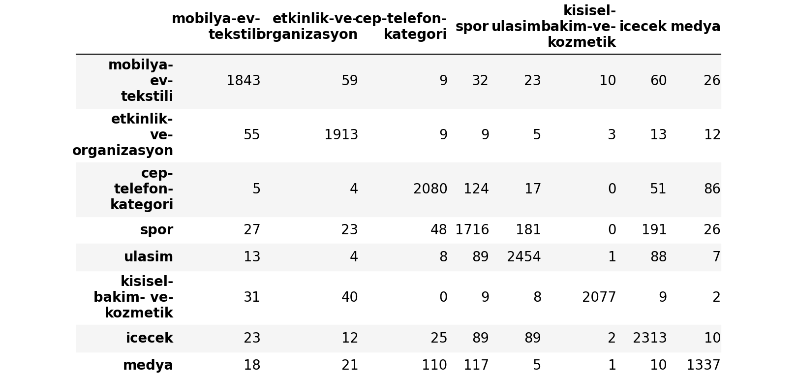

time: 11.4 ms (started: 2023-03-24 13:45:41 +00:00)

We can also visualize the confusion matrix as the ratios of the predictions over the classes. The ratios on the diagonal are the ratios of the correct predictions.

import seaborn as sns
import matplotlib.pyplot as plt
plt.figure(figsize=(7,7))

ax = sns.heatmap(cm_df.iloc[:firstN , 
                            :firstN]/np.sum(cm_df.iloc[:firstN , :firstN]), 
                 annot=True, fmt='.1%', cmap='Blues')

ax.set_title('Confusion Matrix\n\n');
ax.set_xlabel('\nPredicted')
ax.set_ylabel('Actual');

ax.xaxis.set_ticklabels(list(id_to_category.values())[:firstN])
ax.yaxis.set_ticklabels(list(id_to_category.values())[:firstN])

## Display the visualization of the Confusion Matrix.
plt.show()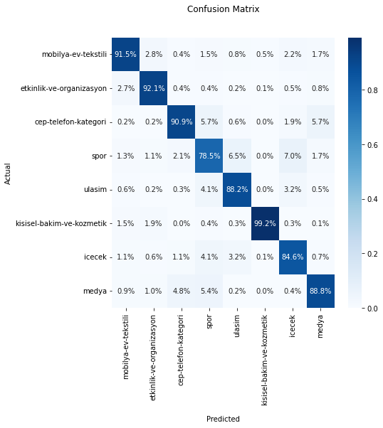

time: 635 ms (started: 2023-03-24 13:44:49 +00:00)

Please, observe the correctly classified sample ratios of each class.

You may need to take some actions for some classes if the correctly predicted sample ratios are relatively low.

Create an End-to-End model

In the code above, we applied the TextVectorization layer to the dataset before feeding text to the model. If you want to make your model capable of processing raw strings (for example, to simplify deploying it), you can include the TextVectorization layer inside your model. You can call this model an End-to-End model.

To do so, you can create a new model using the TextVectorization layer (vectorize_layer) we just trained as the first layer.

end_to_end_model = tf.keras.Sequential([
  vectorize_layer,
  model_LSTM,
  layers.Activation('softmax')
])

end_to_end_model.compile(
    loss=tf.keras.losses.SparseCategoricalCrossentropy(from_logits=False), 
    optimizer="adam", metrics=['accuracy']
)time: 14.3 ms (started: 2023-03-24 13:47:24 +00:00)

Notice that end_to_end_model generates the exact test accuracy using the raw text with the original model accepting preprocessed text.

loss, accuracy = end_to_end_model.evaluate(test_features, test_targets)
print("Test accuracy: ",accuracy)2640/2640 [==============================] - 27s 10ms/step - loss: 1.3495 - accuracy: 0.7986
Test accuracy:  0.7985720634460449
time: 27.5 s (started: 2023-03-24 13:47:28 +00:00)end_to_end_model.summary()Model: "sequential_2"
_________________________________________________________________
 Layer (type)                Output Shape              Param #   
=================================================================
 text_vectorization (TextVec  (None, 40)               0         
 torization)                                                     
                                                                 
 model_LSTM (Functional)     (None, 32)                2194016   
                                                                 
 activation_1 (Activation)   (None, 32)                0         
                                                                 
=================================================================
Total params: 2,194,016
Trainable params: 2,194,016
Non-trainable params: 0
_________________________________________________________________
time: 25 ms (started: 2023-03-24 13:47:59 +00:00)

Let’s observe the prediction of end_to_end_model with the raw text:

examples = [
  "Bir fenomen aracılığı ile Yalova Terma City otel'den arandık. Tatil kazandınız buyurun 16 ocakta gelin dediler. Gittik (2 küçük çocuk, eşim ve annem ), bizi y** adlı kişi karşıladı. Tanıtım yapacağız 4 saat dedi. Daha odamıza bile geçemeden, dinlemeye fırsat vermeden bize oteli gezdirmeye başladılar. Gürültülü, müzik sesli, havasız, kalabalık (Corona olduğu dönemde) bir salonda bize tapulu 1 haftalık arsa sattılar. (psikolojik baskı ile) Tabi o yorgunlukla (amaçları da bu zaten) dinlenmeden bize otelin her detayını anlattılar. Tapumuzu almadan para istediler, güvendik aldık. IBAN numarası otele ait olmayan şahsa 30 bin tl ödedik. 1 gün sonra tapu işlemleri yapılacaktı istemiyoruz tapu, tatil dedik. Kabul etmiyorlar, paramızı vermiyorlar. Ayrıca annemin kaldığı odada ısıtma sistemi çalışmıyordu, çocuk havuzu aşırı pisti, kadınlara ait termal havuz kapalı idi, odada telefon çalışmıyordu ya da bilerek sessize alıyorlar ilgilenmemek için.",
  "5 yıl kullandığım buzdolabım buzluktan şu akıtmaya başladı. Servis geldi içini boşaltın. Lastiklerinden hava alıyor sıcak suyla lastikleri yıkayın dediler. Denileni yaptım. 1 sene olmadan tekrar akıtmaya başladı",
  "Hepsiburada'dan esofman takimi aldık. 18 ocakta yola çıktı ve teslim edildi gözüküyor. Teslim adresi kayınpederimin dükkandı. Ben elemanlar aldı diye düşündüm. Fakat birkaç gün geçti getiren olmadı. Sorunca da kimsenin teslim almadığını öğrendim. Lütfen kargomuzu kime teslim ettiğinizi öğrenin, o gün dağıtım yapan kuryenize sorabilirsiniz. Gereğinin yapılacağını umuyorum, kızıma aldığım bir hediyeydi üzgünüm.",
  "Bimcell tarafıma mesaj atıp 6GB internet Hediye! Evet yazıp 3121'e göndererek kampanyaya katilin,3 gün içinde 30 TL'ye Dost Orta Paket almanız karşılığında haftalık 6GB cepten internet kazanın! Şeklinde mesaj attı dediklerini yerine getirdim paketi yaptım 3121 e Evet yazarak mesaj attım ancak 24.01.2022 de yaptığım işlem hala gerçekleşmedi hediye 6 GB hattıma tanımlanmadı",
  "Instagram'da gözlük marketi hesabı sattığı kalitesiz ürünü geri almıyor. Gözlük çok kötü. Saplar oyuncak desen değil. Oyuncakçıdan alsam çok daha kaliteli olurdu. Bir yazdım iade edebilirsiniz diyor. Sonra yok efendim iademiz yok diyor.",
  "Tamamlayıcı sağlık sigortamı iptal etmek istiyorum fakat ne bankadan ne NN SİGORTA'dan bir tek muhatap bile bulamıyorum. Telefonda dakikalarca tuşlama yapıp bekletiliyor kimsenin cevap verdiği yok. Zaman kaybından başka bir şey değil! İletişim kurabileceğim biri tarafından aranmak istiyorum",
  "Selamlar TOKİ ve emlak yönetimden şikayetimiz var. Kastamonu merkez örencik TOKİ 316 konut 3 gündür kömür gelmedi bir çok blokta kömür bitmiş durumda bu kış zamanında eksi 8 ila 15 derecede yaşlılar hastalar çocuklar bütün herkesi mağdur ettiler. Emlak yönetim 734.60 ton kömür anlaşması yapmış onu da geç yaptığı için zaten yüksek maliyet çıkarmıştı yeni fiyat güncellemesi yapacakmış örneğin bana 6.160 TL nin üzerine fiyat eklenecekmiş bu işi yapan sorumlu kişi veya kişilerin zamanında tedbir almamasının cezasını TOKİ de oturan insanlar çekiyor ya sistem ya da kişiler hatalı"
]

predictions=end_to_end_model.predict(examples)
for pred in predictions:
  print(id_to_category[np.argmax(pred)])1/1 [==============================] - 1s 745ms/step
turizm
otomotiv
internet
internet
gida
bilgisayar
emlak-ve-insaat
time: 794 ms (started: 2023-03-24 13:48:09 +00:00)

Add an Interface with Gradio

!pip install gradio --quiettime: 6.12 s (started: 2023-03-24 13:50:44 +00:00)import gradio as gr

def classify(text):
    pred =end_to_end_model.predict([text])
    return id_to_category[np.argmax(pred)]


demo = gr.Interface(
    fn=classify,
    inputs=gr.inputs.Textbox(lines=5, label="Input Review"),
    outputs=gr.outputs.Textbox(label="Predicted Review Class"),
    examples=examples
)

demo.launch()

Summary

In this part,

we created a Deep Learning model with a Bidirectional LSTM layer to classify text into multi-classes,
we trained and tested the model,
we observed the model performance using Classification Report and Confusion Matrix,
we pointed out the importance of the balanced dataset and the performance of each class.
we created an end-to-end model by integrating the Keras Text Vectorization layer into the final model.
we designed a simple UI with Gradio.

In the next part, we will design another Deep Learning model by using a Transformers Encoder Block.

FULL CODE LINKS:

You can access the complete codes as Colab Notebooks here or using the links given in each video description or you can visit the Murat Karakaya Akademi Github Repo.

YOUTUBE VIDEOS LINKS:

You can watch all these parts on the Murat Karakaya Akademi YouTube channel in ENGLISH or TURKISH.

Comments or Questions?

Please share your Comments or Questions.
Thank you in advance.
Do not forget to check out the next parts!
Take care!

You can access Murat Karakaya Akademi via:

YouTube
Facebook
Instagram
LinkedIn
GitHub
Kaggle
muratkarakaya.net

Saturday, April 8, 2023

Part G: Text Classification with a Recurrent Layer

Photo by Markus Spiske on Unsplash

Part G: Text Classification with A Recurrent Layer

Let’s build a model with a Bidirectional LSTM layer

Important LSTM Parameters

Why do we set return_sequences parameter to true?

Save the trained model

Test

Predictions

Classification Report

Confusion Matrix

Create an End-to-End model

Add an Interface with Gradio

Summary

You can access the complete codes as Colab Notebooks here or using the links given in each video description or you can visit the Murat Karakaya Akademi Github Repo.

YOUTUBE VIDEOS LINKS:

You can watch all these parts on the Murat Karakaya Akademi YouTube channel in ENGLISH or TURKISH.

Comments or Questions?

Please share your Comments or Questions.
Thank you in advance.
Do not forget to check out the next parts!
Take care!

You can access Murat Karakaya Akademi via:

YouTube
Facebook
Instagram
LinkedIn
GitHub
Kaggle
muratkarakaya.net

Social Media Icons

Total Pageviews

Saturday, April 8, 2023

Part G: Text Classification with a Recurrent Layer

Photo by Markus Spiske on Unsplash

Part G: Text Classification with A Recurrent Layer

Let’s build a model with a Bidirectional LSTM layer

Important LSTM Parameters

Why do we set return_sequences parameter to true?

Save the trained model

Test

Predictions

Classification Report

Confusion Matrix

Create an End-to-End model

Add an Interface with Gradio

Summary

You can access the complete codes as Colab Notebooks here or using the links given in each video description or you can visit the Murat Karakaya Akademi Github Repo.

YOUTUBE VIDEOS LINKS:

You can watch all these parts on the Murat Karakaya Akademi YouTube channel in ENGLISH or TURKISH.

Comments or Questions?

Please share your Comments or Questions.Thank you in advance.Do not forget to check out the next parts!Take care!

You can access Murat Karakaya Akademi via:

YouTubeFacebookInstagramLinkedInGitHubKagglemuratkarakaya.net

Please share your Comments or Questions.
Thank you in advance.
Do not forget to check out the next parts!
Take care!

YouTube
Facebook
Instagram
LinkedIn
GitHub
Kaggle
muratkarakaya.net